Gene-centric multiomics clustering

This vignette explains the approach taken by the SplineOmics function: cluster_genes_multiomics. Figure 1 shows the methodological approach.

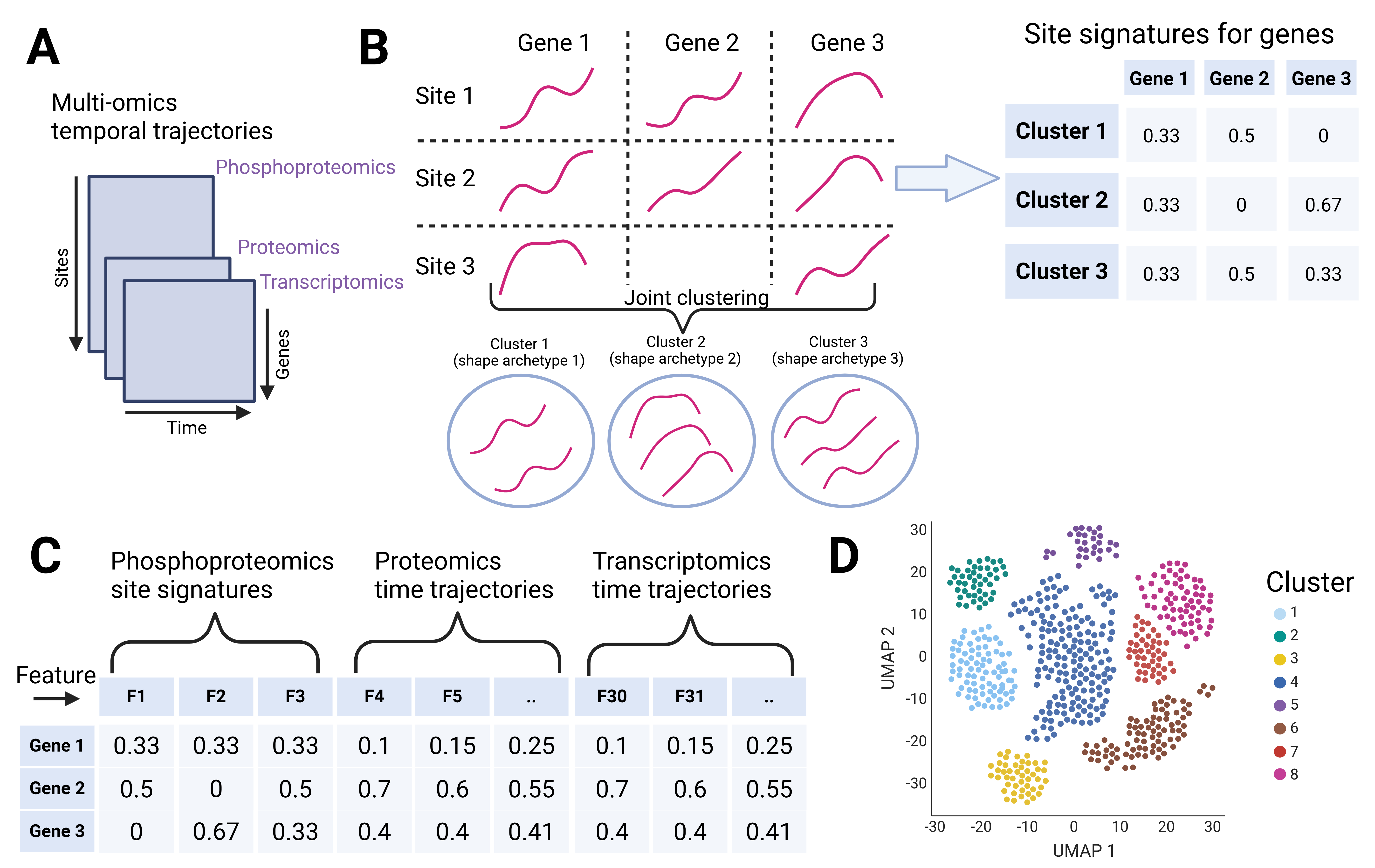
Figure 1: Overview of the gene-centric multi-omics clustering approach. (A) Multi-omics time-series data are collected across several molecular data modalities Some modalities provide a single trajectory per gene, while others contain multiple features that map to the same gene. (B) For modalities with a many-to-one mapping to genes, all feature trajectories are jointly clustered into dynamic pattern groups (shape archetypes). For each gene, the distribution of its features across these pattern groups is summarized as a fixed-length pattern-signature vector. This preserves information from all features without collapsing them and ensures that each gene obtains a standardized representation, regardless of how many features map to it. (C) For every omics modality, a gene-gene distance matrix is computed using the corresponding gene-level trajectories or pattern-signature vectors. This yields one gene×gene distance matrix per modality, each capturing modality-specific similarity between genes. (D) The modality-specific distance matrices are combined into a unified multi-omics distance using user-defined block weights: D(i,j) = Σ w_l * d_l(i,j). The resulting integrated distance matrix reflects multi-modality similarity while preventing any single modality from dominating. (E) Genes are then clustered based on this unified distance to identify coherent multi-omics gene modules.

Here is now shown how to use cluster_genes_multiomics() on a small, synthetic dataset. The example generates multi-omics time-series trajectories, including a many-to-one modality (feature-level measurements mapping to genes), and shows how to assemble the required inputs:

blocks (nested list of block × modality matrices)
block_meta (block-level metadata)
modality_meta (modality-level metadata)

The function returns a named list with two tibbles:

cluster_table: per-gene cluster assignments per block
centroid_info: per-block, per-modality centroid trajectories and within-cluster coherence summaries (and optionally per-member R² vectors)

library(SplineOmics)
library(tibble)
library(ggplot2)

1. Simulate multi-omics time-series data

We generate two blocks (conditions): Constant and Temp_shifted. Each block contains three modalities:

rna (one-to-one; one trajectory per gene)
protein (one-to-one; one trajectory per gene)
phospho (many-to-one; multiple features map to each gene)

The synthetic data uses a small set of canonical temporal shapes and assigns each gene to one latent shape (for simulation only).

set.seed(1)

n_genes <- 40
genes <- paste0("gene", seq_len(n_genes))

n_tp <- 9
t <- seq(0, 1, length.out = n_tp)

.add_noise <- function(x, sd = 0.15) {
  x + rnorm(length(x), mean = 0, sd = sd)
}

.shape_sin  <- function(t) sin(2 * pi * t)
.shape_cos  <- function(t) cos(2 * pi * t)
.shape_up   <- function(t) 2 * t - 1
.shape_down <- function(t) 1 - 2 * t
.shape_peak <- function(t) exp(-((t - 0.5) / 0.18)^2) * 2 - 1

shapes <- list(
  S1 = .shape_sin(t),
  S2 = .shape_cos(t),
  S3 = .shape_up(t),
  S4 = .shape_down(t),
  S5 = .shape_peak(t)
)

true_k <- 5
gene_group <- sample(seq_len(true_k), n_genes, replace = TRUE)

1.1 Simulate RNA and protein (one-to-one)

RNA is simulated from the latent shapes with noise. Protein is simulated as a lagged and scaled version of RNA (with additional noise), mimicking delayed protein dynamics relative to transcripts.

.simulate_one_to_one <- function(genes, shapes, gene_group, noise_sd = 0.18) {
  n_genes <- length(genes)
  n_tp <- length(shapes[[1]])
  X <- matrix(
    NA_real_,
    nrow = n_genes,
    ncol = n_tp,
    dimnames = list(genes, paste0("tp", seq_len(n_tp)))
  )

  for (i in seq_len(n_genes)) {
    k <- gene_group[i]
    base <- shapes[[k]]
    X[i, ] <- .add_noise(base, sd = noise_sd)
  }

  X
}

rna_constant <- .simulate_one_to_one(
  genes = genes,
  shapes = shapes,
  gene_group = gene_group,
  noise_sd = 0.16
)

rna_temp <- rna_constant
for (i in seq_len(n_genes)) {
  k <- gene_group[i]
  warp <- if (k %in% c(1, 5)) 0.25 else 0.10
  rna_temp[i, ] <- .add_noise(shapes[[k]] + warp * t, sd = 0.16)
}
rownames(rna_temp) <- genes
colnames(rna_temp) <- colnames(rna_constant)

.lag_vec <- function(x, lag = 1) {
  if (lag <= 0) return(x)
  c(rep(x[1], lag), x[seq_len(length(x) - lag)])
}

protein_constant <- rna_constant
for (i in seq_len(n_genes)) {
  v <- rna_constant[i, ]
  protein_constant[i, ] <- .add_noise(0.8 * .lag_vec(v, lag = 1), sd = 0.18)
}
rownames(protein_constant) <- genes
colnames(protein_constant) <- colnames(rna_constant)

protein_temp <- rna_temp
for (i in seq_len(n_genes)) {
  v <- rna_temp[i, ]
  protein_temp[i, ] <- .add_noise(0.85 * .lag_vec(v, lag = 1), sd = 0.18)
}
rownames(protein_temp) <- genes
colnames(protein_temp) <- colnames(rna_temp)

1.2 Simulate phospho features (many-to-one)

For each gene, we create 1–4 phospho features. Each feature follows the gene’s latent shape with feature-specific perturbations. Rows are named <gene>_<feature> to encode the many-to-one mapping.

.simulate_many_to_one <- function(genes, shapes, gene_group,
                                  min_feat = 1, max_feat = 4,
                                  noise_sd = 0.20) {
  feat_counts <- sample(min_feat:max_feat, length(genes), replace = TRUE)

  feat_ids <- unlist(
    mapply(
      function(g, n) paste0(g, "_p", seq_len(n)),
      genes, feat_counts,
      SIMPLIFY = FALSE
    ),
    use.names = FALSE
  )

  n_feat <- length(feat_ids)
  n_tp <- length(shapes[[1]])

  X <- matrix(
    NA_real_,
    nrow = n_feat,
    ncol = n_tp,
    dimnames = list(feat_ids, paste0("tp", seq_len(n_tp)))
  )

  idx <- 0L
  for (i in seq_along(genes)) {
    k <- gene_group[i]
    base <- shapes[[k]]

    n_f <- feat_counts[i]
    for (j in seq_len(n_f)) {
      idx <- idx + 1L

      amp <- runif(1, 0.7, 1.3)
      drift <- runif(1, -0.25, 0.25)
      X[idx, ] <- .add_noise(amp * base + drift * t, sd = noise_sd)
    }
  }

  X
}

phospho_constant <- .simulate_many_to_one(genes, shapes, gene_group)

phospho_temp <- phospho_constant
for (i in seq_len(nrow(phospho_temp))) {
  g <- sub("_.*$", "", rownames(phospho_temp)[i])
  gi <- match(g, genes)
  k <- gene_group[gi]
  bump <- if (k %in% c(2, 4)) 0.35 else 0.12
  phospho_temp[i, ] <- .add_noise(phospho_temp[i, ] + bump * t, sd = 0.20)
}

2. Build inputs for `cluster_genes_multiomics()`

Each block is a list of modality matrices. block_meta defines the number of gene clusters per block and the result category. modality_meta specifies, per (block × modality), whether a modality is one-to-one (layer_k = NA) or many-to- one (layer_k positive), and the relative layer weights.

blocks <- list(
  Constant = list(
    rna     = rna_constant,
    protein = protein_constant,
    phospho = phospho_constant
  ),
  Temp_shifted = list(
    rna     = rna_temp,
    protein = protein_temp,
    phospho = phospho_temp
  )
)

block_clusters <- list(
    Constant     = 5L,
    Temp_shifted = 5L
)

modality_meta <- data.frame(
  block   = rep(c("Constant", "Temp_shifted"), each = 3),
  layer   = rep(c("rna", "protein", "phospho"), times = 2),
  layer_k = c(NA_real_, NA_real_, 4,
              NA_real_, NA_real_, 4),
  layer_w = c(1, 1, 1,
              1, 1, 1)
)

3. Run gene-centric multi-omics clustering

The function returns a list with cluster_table and centroid_info.

res <- cluster_genes_multiomics(
  blocks        = blocks,
  block_clusters = block_clusters,
  modality_meta = modality_meta,
  gene_mode     = "intersection",
  verbose       = TRUE
)
#> [cluster_genes_multiomics] Block 1/2: 'Constant'
#>   [block 'Constant'] building gene-level layer matrices...
#>   [block 'Constant'] computing and combining layer-wise distance matrices...
#>   [block 'Constant'] clustering genes (k = 5)...
#> [cluster_genes_multiomics] Block 2/2: 'Temp_shifted'
#>   [block 'Temp_shifted'] building gene-level layer matrices...
#>   [block 'Temp_shifted'] computing and combining layer-wise distance matrices...
#>   [block 'Temp_shifted'] clustering genes (k = 5)...
#> [cluster_genes_multiomics] total runtime: 0.031 secs

cluster_table <- res$cluster_table
centroid_info <- res$centroid_info

4. Inspect `cluster_table`

cluster_table contains one row per gene and one cluster assignment column per block. For time-effect blocks (result category 1), these columns are named cluster_<cond>.

cluster_table
#> # A tibble: 40 × 3
#>    gene   Constant Temp_shifted
#>    <chr>     <int>        <int>
#>  1 gene1         5            3
#>  2 gene10        5            3
#>  3 gene11        2            4
#>  4 gene12        2            4
#>  5 gene13        3            2
#>  6 gene14        3            2
#>  7 gene15        5            3
#>  8 gene16        2            4
#>  9 gene17        2            4
#> 10 gene18        5            3
#> # ℹ 30 more rows

table(cluster_table$cluster_Constant, useNA = "ifany")
#> Warning: Unknown or uninitialised column: `cluster_Constant`.
#> < table of extent 0 >
table(cluster_table$cluster_Temp_shifted, useNA = "ifany")
#> Warning: Unknown or uninitialised column: `cluster_Temp_shifted`.
#> < table of extent 0 >

5. Inspect `centroid_info`

centroid_info summarizes, for each (block × modality × cluster), the centroid trajectory (list-column) and coherence metrics (mean and sd of per-gene R²). If your implementation stores per-member R² values in r2_member, you can use those to inspect outliers within a cluster.

centroid_info
#> # A tibble: 30 × 11
#>    block    modality modality_type cluster n_genes_cluster n_genes_used coverage
#>    <chr>    <chr>    <chr>           <int>           <int>        <int>    <dbl>
#>  1 Constant rna      one_to_one          1               4            4        1
#>  2 Constant rna      one_to_one          2               7            7        1
#>  3 Constant rna      one_to_one          3              10           10        1
#>  4 Constant rna      one_to_one          4               8            8        1
#>  5 Constant rna      one_to_one          5              11           11        1
#>  6 Constant protein  one_to_one          1               4            4        1
#>  7 Constant protein  one_to_one          2               7            7        1
#>  8 Constant protein  one_to_one          3              10           10        1
#>  9 Constant protein  one_to_one          4               8            8        1
#> 10 Constant protein  one_to_one          5              11           11        1
#> # ℹ 20 more rows
#> # ℹ 4 more variables: mean_R2 <dbl>, sd_R2 <dbl>, r2_member <I<list>>,
#> #   centroid <I<list>>

subset(
  centroid_info,
  block == "Constant" & modality == "rna",
  select = c("block", "modality", "cluster", "n_genes_used",
             "coverage", "mean_R2", "sd_R2")
)
#> # A tibble: 5 × 7
#>   block    modality cluster n_genes_used coverage mean_R2   sd_R2
#>   <chr>    <chr>      <int>        <int>    <dbl>   <dbl>   <dbl>
#> 1 Constant rna            1            4        1   0.965 0.0127 
#> 2 Constant rna            2            7        1   0.972 0.00939
#> 3 Constant rna            3           10        1   0.967 0.0163 
#> 4 Constant rna            4            8        1   0.960 0.0142 
#> 5 Constant rna            5           11        1   0.966 0.0181

5.1 Plot a centroid trajectory

Centroids are stored as numeric vectors in a list-column. Use [[ ]] to extract a single centroid and plot it.

ci_rna_const <- subset(
  centroid_info,
  block == "Constant" & modality == "rna"
)

i <- 1

centroid_df <- data.frame(
  time  = seq_along(ci_rna_const$centroid[[i]]),
  value = ci_rna_const$centroid[[i]]
)

ggplot(centroid_df, aes(x = time, y = value)) +
  geom_line(linewidth = 0.9) +
  geom_point(size = 1.8) +
  labs(
    title = paste(
      "Centroid trajectory:",
      ci_rna_const$block[i],
      ci_rna_const$modality[i],
      "cluster", ci_rna_const$cluster[i]
    ),
    x = "Spline / time point",
    y = "Centroid (z-scored)"
  ) +
  theme_bw()

5.2 Inspect per-member R² values

If your centroid_info includes a list-column r2_member (named numeric vectors of per-gene R²), you can examine the distribution and identify low-fit genes. If the column does not exist, this section will be skipped.

if ("r2_member" %in% names(ci_rna_const)) {

  i <- 1
  r2 <- ci_rna_const$r2_member[[i]]

  print(head(r2))
  print(summary(r2))

  r2_df <- data.frame(
    gene = names(r2),
    R2   = unname(r2)
  )

  p <- ggplot(r2_df, aes(x = R2)) +
    geom_histogram(
      bins = 15,
      colour = "black",
      fill = "grey80"
    ) +
    labs(
      title = paste(
        "Per-gene R² to centroid:",
        ci_rna_const$block[i],
        ci_rna_const$modality[i],
        "cluster", ci_rna_const$cluster[i]
      ),
      x = expression(R^2),
      y = "Gene count"
    ) +
    theme_bw()

  print(p)

  bad <- r2_df$gene[r2_df$R2 < 0.2]
  print(bad)

} else {
  message("No r2_member column found in centroid_info (optional feature).")
}
#>    gene28     gene6     gene8     gene9 
#> 0.9609069 0.9510050 0.9808992 0.9690602 
#>    Min. 1st Qu.  Median    Mean 3rd Qu.    Max. 
#>  0.9510  0.9584  0.9650  0.9655  0.9720  0.9809

#> character(0)

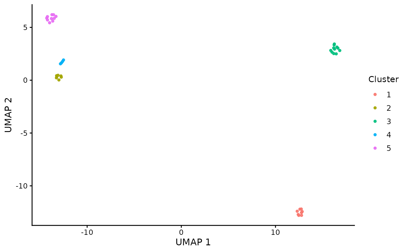
Session Info

#> R version 4.5.2 (2025-10-31)
#> Platform: x86_64-pc-linux-gnu
#> Running under: Ubuntu 22.04.5 LTS
#> 
#> Matrix products: default
#> BLAS:   /usr/lib/x86_64-linux-gnu/blas/libblas.so.3.10.0 
#> LAPACK: /usr/lib/x86_64-linux-gnu/lapack/liblapack.so.3.10.0  LAPACK version 3.10.0
#> 
#> locale:
#>  [1] LC_CTYPE=en_US.UTF-8       LC_NUMERIC=C              
#>  [3] LC_TIME=de_AT.UTF-8        LC_COLLATE=en_US.UTF-8    
#>  [5] LC_MONETARY=de_AT.UTF-8    LC_MESSAGES=en_US.UTF-8   
#>  [7] LC_PAPER=de_AT.UTF-8       LC_NAME=C                 
#>  [9] LC_ADDRESS=C               LC_TELEPHONE=C            
#> [11] LC_MEASUREMENT=de_AT.UTF-8 LC_IDENTIFICATION=C       
#> 
#> time zone: Europe/Vienna
#> tzcode source: system (glibc)
#> 
#> attached base packages:
#> [1] stats     graphics  grDevices datasets  utils     methods   base     
#> 
#> other attached packages:
#> [1] ggplot2_3.5.2     tibble_3.3.0      SplineOmics_0.4.2
#> 
#> loaded via a namespace (and not attached):
#>   [1] bitops_1.0-9             Rdpack_2.6.4             pbapply_1.7-2           
#>   [4] writexl_1.5.4            rlang_1.1.6              magrittr_2.0.3          
#>   [7] clue_0.3-66              GetoptLong_1.0.5         matrixStats_1.5.0       
#>  [10] compiler_4.5.2           reshape2_1.4.4           png_0.1-8               
#>  [13] systemfonts_1.2.3        vctrs_0.6.5              stringr_1.5.1           
#>  [16] pkgconfig_2.0.3          shape_1.4.6.1            crayon_1.5.3            
#>  [19] fastmap_1.2.0            backports_1.5.0          labeling_0.4.3          
#>  [22] utf8_1.2.6               caTools_1.18.3           rmarkdown_2.29          
#>  [25] nloptr_2.2.1             ragg_1.4.0               purrr_1.1.0             
#>  [28] xfun_0.52                cachem_1.1.0             jsonlite_2.0.0          
#>  [31] progress_1.2.3           EnvStats_3.1.0           remaCor_0.0.18          
#>  [34] gmp_0.7-5                BiocParallel_1.42.1      broom_1.0.8             
#>  [37] parallel_4.5.2           prettyunits_1.2.0        cluster_2.1.8.1         
#>  [40] R6_2.6.1                 stringi_1.8.7            bslib_0.9.0             
#>  [43] RColorBrewer_1.1-3       limma_3.64.1             car_3.1-3               
#>  [46] boot_1.3-31              ClusterR_1.3.3           numDeriv_2016.8-1.1     
#>  [49] jquerylib_0.1.4          Rcpp_1.1.0               iterators_1.0.14        
#>  [52] knitr_1.50               base64enc_0.1-3          IRanges_2.42.0          
#>  [55] Matrix_1.7-3             splines_4.5.2            tidyselect_1.2.1        
#>  [58] rstudioapi_0.17.1        abind_1.4-8              yaml_2.3.10             
#>  [61] doParallel_1.0.17        gplots_3.2.0             codetools_0.2-19        
#>  [64] plyr_1.8.9               lmerTest_3.1-3           lattice_0.22-5          
#>  [67] withr_3.0.2              Biobase_2.68.0           evaluate_1.0.4          
#>  [70] desc_1.4.3               zip_2.3.3                circlize_0.4.16         
#>  [73] pillar_1.11.0            BiocManager_1.30.26      carData_3.0-5           
#>  [76] KernSmooth_2.23-26       checkmate_2.3.3          renv_1.1.5              
#>  [79] foreach_1.5.2            stats4_4.5.2             reformulas_0.4.1        
#>  [82] generics_0.1.4           rprojroot_2.1.1          S4Vectors_0.46.0        
#>  [85] hms_1.1.3                scales_1.4.0             aod_1.3.3               
#>  [88] minqa_1.2.8              gtools_3.9.5             RhpcBLASctl_0.23-42     
#>  [91] glue_1.8.0               tools_4.5.2              fANCOVA_0.6-1           
#>  [94] variancePartition_1.38.0 lme4_1.1-37              mvtnorm_1.3-3           
#>  [97] fs_1.6.6                 grid_4.5.2               tidyr_1.3.1             
#> [100] rbibutils_2.3            colorspace_2.1-1         nlme_3.1-168            
#> [103] Formula_1.2-5            cli_3.6.5                textshaping_1.0.1       
#> [106] svglite_2.2.1            ComplexHeatmap_2.24.1    dplyr_1.1.4             
#> [109] corpcor_1.6.10           gtable_0.3.6             sass_0.4.10             
#> [112] digest_0.6.37            BiocGenerics_0.54.0      pbkrtest_0.5.4          
#> [115] ggrepel_0.9.6            rjson_0.2.23             htmlwidgets_1.6.4       
#> [118] farver_2.1.2             htmltools_0.5.8.1        pkgdown_2.1.3           
#> [121] lifecycle_1.0.4          here_1.0.1               GlobalOptions_0.1.2     
#> [124] statmod_1.5.0            MASS_7.3-65

Gene-centric multiomics clustering

Thomas Rauter

19 January, 2026